Hierarchical Mixture Model for Single Cell Sequencing I
One of my favorite parts of my job is that I am able to spend 1 day per week focusing on applying our hierarchical mixture modeling technology to genomic applications. I’ve been working closely with the Ramiz Somjee on applying our technology to scRNA sequencing data.
TLDR: Why I’m Excited
Current scRNA pipelines rely on a heuristic driven 2-step process. First some form of filtering+dimensionality reduction, followed by a clustering step, followed by either manual labeling of these clusters or a classification model to learn/apply annotation to this data.
Our technology can model this entire pipeline in as a single unified joint probabilty distribution with 3 branches. We have a topic branch that learns a probability distribution across genes for each topic, a cell branch that learns a probabilty distribution across topics for each cell, and a classification branch that learns regression weights for each cell’s topic distribution.
This is powerful because our topics are jointly modeling both the unsupervised co-occurance information along with any annotations provided. This structure enables not only robust, few-shot classification but also extremely granular explainability.
First Experiment
We took an already annotated dataset that Ramiz was extremely familiar with to evaluate (1) whether our model was capable to learning the annotations and (2) whether the genes that comprised the predictive topics lined up with Ramiz’s extensive manual annotation process.
The model actually worked better than I could have hoped. We trained the model on 150 labels for 12 different cell types. We then evaluated the model on 2000 held out datapoints. Our model mislabelled only 3/2000 examples in the test set. We didn’t dig too deep into the model performance beyond that, since this was more just a validation experiement.
What I was really excited to dig into was the explanatory analysis. Our model uses a error-tolerant variant of the sparsity-inducing Finish Horseshoe prior that we call the Santa Barbara Horseshoe. This prior enables our model, with only a few examples, to confidently separate meaningful parameters from noisy ones.
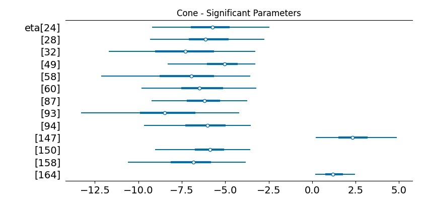
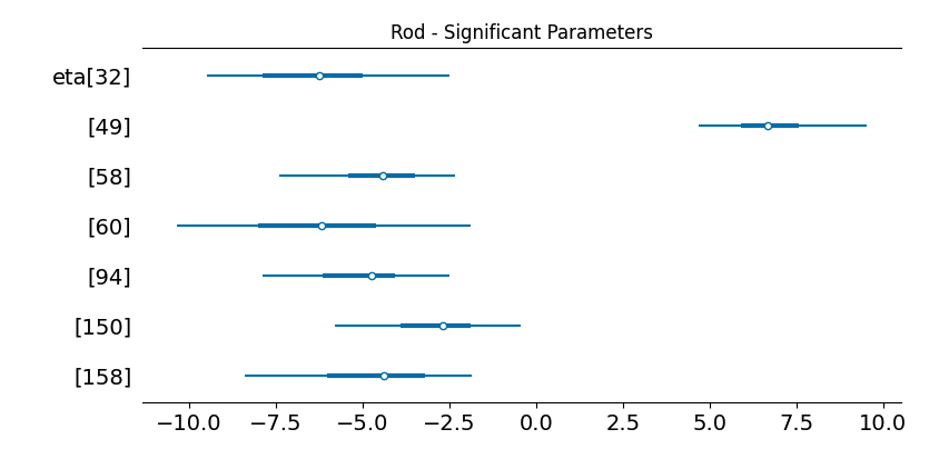
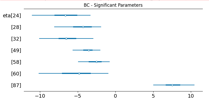
What’s really cool is now for any of the predictive topics, we can dig into the genes that comprise it:
Topic 49: Predictive of Rod
['Sag', 'Gngt1', 'Rho', 'mt-Atp6', 'Pdc', 'Mir124-2hg', 'Prph2',
'mt-Co2', 'Unc119', 'Pde6g', 'Tma7', 'Rom1', 'Ubb', 'Nr2e3',
'Rpl26', 'Hsp90aa1', 'H3f3b', 'mt-Cytb', 'Gapdh', 'H3f3a',
'Rpgrip1', 'Pkm', 'Rp1', 'mt-Co3', 'Gnb1', 'mt-Co1', 'Ckb']
These genes line up really exactly with Ramiz’s manual annotation. The difference was that this pipeline was fully automatic.
Next Steps
While I believe there is a lot of value to the explainble components of this model, we are going to focus on classification because it is much easier to quantitatively evaluate and can also solve a real pain point for the scRNA research community. I described the current painstaking process of annotating scRNA sequences that is extremely manual, heuristic, and time consuming. The reason for this current process is current classification methods do not generalize across experiments: batch effects throw off normal statistics based classification and clustering models.
Our model provides a number of avenues to handle batch effects. Our hope is that it works out of the box, but we also have hierarchical levers we can pull to factor batch effects directly into our model structure. We plan to take 35 annotated datasets of mouse eye scRNA sequences, train our model on one of them, and evaluate it’s performance on the other 34. Our model’s performancew ill determine the next steps from there, but I’m extremely excited and optimistic based on our initial set of results.